09/18/2019: Introduction to Machine Learning Lecture with Prof. Rogan
To start of this meeting, we officially (and unanimously!) ratified the LML Constitution, which can be found here. For quorum purposes, we had 16 active members in attendance. There were 16 in favor of ratifying the Constitution and 0 opposed.
After the ratification, Professor Rogan briefly reminded us of his lecture from two weeks ago, which recounted the decision boundary problem as outlined in “Elements of Statistical Learning” by Hastie, et. al. (see Chapter 11). The effectiveness of the boundary between the two datasets was measured by the residual sum squared, which Professor Rogan also reviewed.
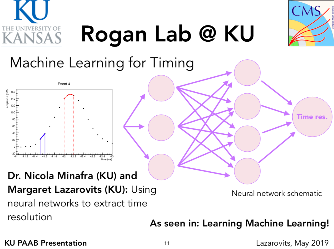
Next, he pivoted the conversation to neural networks. This form of machine learning is focused on finding an expansion of the prediction in terms of basis functions. This expansion can be thought of as similar to a Fourier Transform. A discrete Fourier Transform (DFT) expands a function in terms of a linear sum of sines and cosines. The coefficients of these sine/cosine terms are similar to the weights applied to the output of each neural network node. The nodes in a neural network can be thought of as the frequencies in a Fourier Transform. However, unlike a DFT, we don’t need an infinite number of nodes to approximate a function. Instead, a neural network makes use of multiple layers of nodes, as well as making the nodes functions, instead of frequencies.
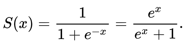
These functions at the nodes are called activation functions. Their nonlinear nature make them particularly adept at describing complex systems. One example of an activation function is the sigmoid, or logisitic functin that was introducted in 1989. It was shown with this activation function that you can approximate any reasonably well behaved function with only two hidden layers of nodes. This particular function is also known as the universal approximation function, although you can use other activation functions to approximate functions with the same number of hidden layers. Other activation functions include the widely-used rectified linear unit (ReLU) function and the softmax function.
Because of these nonlinear activation functions, neural networks are just nonlinear functions stacked on top of each other to create more complex models. When we run input data through a neural network, what the network is doing is learning the weights, or the connections of one node to another. The network recognizes some connections as important, and weights them more heavily, while other connections are deemed less important and their weight can tend to zero.
The way a network learns these weights is by minimizing a loss or cost function with respect to the weights. In our case, the loss function we want to minimize is the residual sum squared (RSS) function. When the input data is sent through the neural network, the network calculates the gradient (partial derivative in every dimension) of the RSS function with respect to the weights. The network then takes a step in the negative gradient direction, updating the weights accordingly, in an attempt to reach a minimum of the loss function. This is why neural networks are called feedforward backpropagating networks. The data is fed forward through the network while the updated weights are propagated backwards through the chain rule of the partial derivatives (gradient).
When it comes to designing a neural network, there is no right answer. In fact, there are many things you can customize including your input data and labels (output), activation functions, number of layers and number of nodes in each layer, which nodes are connected, and the list goes on. However, one thing to keep in mind when training a neural network is that you should have a validation dataset in addition to your training and test set. This validation set is independent from but identically distributed to the training set. It helps make sure that you aren’t strictly training your network to your training set that you can’t generalize the model to more data. When a neural network trains to learn all the nuances to the training set and has little generalizability, it is called overfitting. The capacity, or complexity, of the neural network means that the model has more parameters and therefor higher variance, less variance, and is more likely to overfit the data. However, if a model is too general, with low variance and high bias, you could poorly fit indepedent but identically distributed datasets, as well as your training set. This is known as underfitting, when the model is too general. Therefore, it is important to strike a balance between capacity and generalizability when training a model.
Stopping criteria in the neural network can address the issue of overfitting. When the network passes through one epoch, it goes through one round of updating the weights, and it takes a step in the negative gradient direction, then it repeats. If you can train the network to stop when it starts to take steps up the loss function, this may reduce overfitting. However, it is also good to be able to find a global minimum, not just a local minimum. In order to find this global minimum, it may help to increase the capacity of the network.
Some things to think about when choosing your network architecture are enumerated in Hastie, et. al. Chapter 11. These following aspects are discussed in more detail there: starting values of weights, preprocessing inputs, minimization methods, regularization, and network architecture.
Here are notes taken from this session, provided by Emily Aresenault.
